Abstract
One day, you might have a situation where you are required to update a sheet using Google Apps Script when the cell values retrieved by IMPORTRANGE are changed. This report introduces a workaround for achieving this situation.
Introduction
Google Apps Script can be executed by several triggers. Ref When a cell in a Google Spreadsheet is manually edited, a function of Google Apps Script can be executed by detecting this edit. In most cases, the OnEdit trigger trigger of the simple trigger or the installable trigger is used. When the OnEdit trigger is used, a function can be executed by manually editing a cell. When the function is executed, the function can be run by giving the event object including the information about the edited cell.
Here, there is an important point. The OnEdit trigger is fired only when a cell is manually edited. For example, when a cell is edited by a script and a formula, the OnEdit trigger is not fired. In the case that a cell is edited by a script, the time when the script is run can be used as a trigger. On the other hand, in the case that a cell is updated by a formula, this cannot be directly detected by the OnEdit trigger. This is the current specification. However, there might be a situation where you are required to run a script when a cell is updated by a formula. This report introduces a workaround for achieving this situation.
Here, as a sample situation, I would like to introduce a workaround in which a script is run using the OnEdit trigger when the cell values retrieved with IMPORTRANGE are changed. IMPORTRANGE is one of the sample situations for explaining this workaround. This workaround introduced in this report can be also used for detecting the change of not only IMPORTRANGE but also other formulas. I sometimes saw questions related to this situation in Stackoverflow. So, I thought that when this workaround is introduced, it might be useful for the users.
Principle
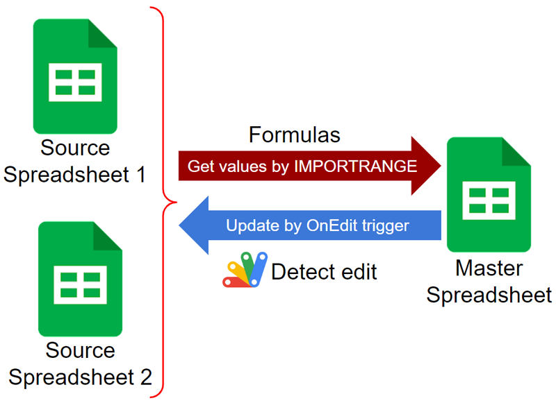
The 2 key factors for achieving this workaround are as follows.
- OnEdit trigger is fired when a cell is manually edited.
- The installable trigger can be also installed by a Google Apps Script project different from the target Google Apps Script project.
In the current stage, unfortunately, even when the value of a formula in a cell is changed by recalculating, the OnEdit trigger is not fired because of the current specification. However, it is considered that when the cell of the origin for recalculating the formula is manually edited, the OnEdit trigger can be used by detecting the cell. This workaround uses this situation.
In the case of IMPORTRANGE, the target Spreadsheet is usually different from the active Spreadsheet. In order to detect the origin cells in the target Spreadsheet, the installable OnEdit trigger is used. The installable OnEdit trigger can be also set from a Google Apps Script project outside of the container-bound script of the target Spreadsheet. This specification is also used in this workaround.
Sample situation
The sample situation is shown in the following image.
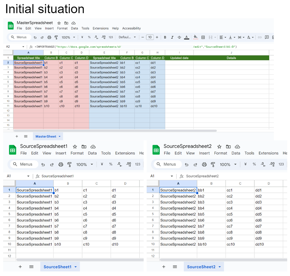
The details of this sample situation is as follows.
-
There are 3 Spreadsheets like “MasterSpreadsheet”, “SourceSpreadsheet1”, and “SourceSpreadsheet2”.
-
A sheet “MasterSheet” in “MasterSpreadsheet” has following 2 formulas.
=IMPORTRANGE("https://docs.google.com/spreadsheets/d/{spreadsheetId of SourceSpreadsheet1}/edit","SourceSheet1!A1:D")in cell “A2”=IMPORTRANGE("https://docs.google.com/spreadsheets/d/{spreadsheetId of SourceSpreadsheet2}/edit","SourceSheet2!A1:D")in cell “E2”
-
Data is retrieved from 2 Spreadsheets of “SourceSpreadsheet1”, and “SourceSpreadsheet2” to “MasterSheet” in “MasterSpreadsheet”.
-
“SourceSheet1!A1:D” in “SourceSpreadsheet1” and “SourceSheet2!A1:D” in “SourceSpreadsheet2” are manually edited.
-
When the cell values of
=IMPORTRANGE("https://docs.google.com/spreadsheets/d/{spreadsheetId of SourceSpreadsheet1}/edit","SourceSheet1!A1:D")in cell “A2” and=IMPORTRANGE("https://docs.google.com/spreadsheets/d/{spreadsheetId of SourceSpreadsheet2}/edit","SourceSheet2!A1:D")in cell “E2” are updated, it is required to put the updated date to column “I” and put the update details to column “J”.
In this report, this situation is achieved using Google Apps Script as the sample goal of this report.
IMPORTANT
This report introduces the workaround for achieving the above sample goal using a simple script as the methodology. So, when you want to use this workaround to your actual situation, I thin that the script is required to be prepared for your actual situation. Please be careful about this.
Usage
In this section, it introduces the sample script for achieving the above goal. In order to test this workaround, please do the following flow.
Prepare Spreadsheets
In this sample, 3 Spreadsheets are used. Here, I prepared a script for creating the sample Spreadsheets of this report as follows.
Please access to https://script.new. By this, the script editor is opened as a new standalone script. Here, copy and paste the following script to the script editor and please give a filename, set your folder ID to folderId, and save the script.
And, please run createSamples() with the script editor. By this, the sample Spreadsheets for using this workaround are created in
the folder of folderId.
function createSamples() {
  const folderId = "###"; // Please set your folder ID. The sample Spreadsheets are created to this folder.

  // Create MasterSpreadsheet.
  const header = [
    "Spreadsheet title",
    "Column B",
    "Column C",
    "Column D",
    "Spreadsheet title",
    "Column B",
    "Column C",
    "Column D",
    "Updated date",
    "Details",
  ];
  const ss1 = SpreadsheetApp.create("MasterSpreadsheet");
  const sheet1 = ss1.getSheets()[0].setName("MasterSheet");
  sheet1.appendRow(header);

  // Create SourceSpreadsheets.
  const ar = [
    { title: "SourceSpreadsheet1", sheetName: "SourceSheet1" },
    { title: "SourceSpreadsheet2", sheetName: "SourceSheet2" },
  ];
  const sss = ar.map(({ title, sheetName }, i) => {
    const ss2 = SpreadsheetApp.create(title);
    const sheet2 = ss2.getSheets()[0].setName(sheetName);
    const k = i + 1;
    const values = [...Array(10)].map((_, i) => [
      title,
      ...["a", "b", "c"].map((e) => `${Array(k).fill(e).join("")}${k}`),
    ]);
    sheet2.getRange(1, 1, values.length, values[0].length).setValues(values);
    return ss2;
  });

  // Move Spreadsheets to folder.
  const folder = DriveApp.getFolderById(folderId || "root");
  [ss1, ...sss].forEach((e) => DriveApp.getFileById(e.getId()).moveTo(folder));

  // Set formulas to MasterSpreadsheet.
  const token = ScriptApp.getOAuthToken();
  const cells = ["A2", "E2"];
  sss.forEach((e, i) => {
    sheet1
      .getRange(cells[i])
      .setFormula(`=IMPORTRANGE("${e.getUrl()}","SourceSheet${i + 1}!A1:D")`);
    const url = `https://docs.google.com/spreadsheets/d/${ss1.getId()}/externaldata/addimportrangepermissions?donorDocId=${e.getId()}`;
    UrlFetchApp.fetch(url, {
      url,
      method: "post",
      headers: { Authorization: `Bearer ${token}` },
      muteHttpExceptions: true,
    });
  });

  console.log([ss1, ...sss].map((e) => ({ [e.getName()]: e.getId() }))); // You can see the Spreadsheet ID of each Spreadsheet.
}
When you run createSamples(), 3 Spreadsheets are created. When you open “MasterSpreadsheet”, “SourceSpreadsheet1”, and “SourceSpreadsheet2”, you can see the Spreadsheet shown in “Sample situation”. These Spreadsheets are used for testing the following script.
Sample script
Please copy and paste the following script to the script editor of “MasterSpreadsheet”. I think that in this method, the standalone script can be also used. But, in this report. the container-bound script of “MasterSpreadsheet” is used.
Before you run this script, please set masterSpreadsheetId, sourceSpreadsheet1Id, and sourceSpreadsheet2Id.
// Please set your values to this function.
function variables_() {
  const masterSpreadsheetId = "###"; // Please set spreadsheet ID of "MasterSpreadsheet".
  const masterSheetName = "MasterSheet";

  const sourceSpreadsheet1Id = "###"; // Please set spreadsheet ID of "SourceSpreadsheet1".
  const sourceSpreadsheet1Range = "SourceSheet1!A1:D";

  const sourceSpreadsheet2Id = "###"; // Please set spreadsheet ID of "SourceSpreadsheet2".

  const sourceSpreadsheet2Range = "SourceSheet2!A1:D";

  return {
    master: { masterSpreadsheetId, masterSheetName },
    sources: [
      { ssId: sourceSpreadsheet1Id, a1Notation: sourceSpreadsheet1Range },
      { ssId: sourceSpreadsheet2Id, a1Notation: sourceSpreadsheet2Range },
    ],
  };
}

// This function is automatically run when the cell of source Spreadsheet 1 or source Spreadsheet 2 is edited.
// Please don't directly run this function.
function installedOnEdit(e) {
  if (!e)
    throw new Error(
      "This function is automatically run when the cell of source Spreadsheet 1 or source Spreadsheet 2 is edited. Please don't directly run this function."
    );
  const lock = LockService.getScriptLock();
  if (lock.tryLock(350000)) {
    try {
      const {
        master: { masterSpreadsheetId, masterSheetName },
        sources,
      } = variables_();
      const { range, source } = e;
      const { a1Notation } = sources.find(({ ssId }) => ssId == source.getId());
      const srcRange = source.getRange(a1Notation);
      const sheet = range.getSheet();
      const editedSheetName = sheet.getSheetName();
      if (
        range.columnStart > srcRange.getNumColumns() ||
        editedSheetName != srcRange.getSheet().getSheetName()
      )
        return;
      const details = `row ${range.rowStart} and column ${range.columnStart} in "${editedSheetName}" was edited.`;
      const masterSheet =
        SpreadsheetApp.openById(masterSpreadsheetId).getSheetByName(
          masterSheetName
        );
      masterSheet
        .getRange(range.rowStart + 1, 9, 1, 2)
        .setValues([[new Date(), details]]);
    } catch ({ stack }) {
      console.error(stack);
    } finally {
      lock.releaseLock();
      console.log("Done");
    }
  } else {
    console.error("Timeout");
  }
}

// Please run this function.
function main() {
  const functionName = "installedOnEdit";
  ScriptApp.getProjectTriggers().forEach((t) => {
    if (t.getHandlerFunction() == functionName) {
      ScriptApp.deleteTrigger(t);
    }
  });
  const { sources } = variables_();
  sources.forEach(({ ssId }) =>
    ScriptApp.newTrigger(functionName)
      .forSpreadsheet(SpreadsheetApp.openById(ssId))
      .onEdit()
      .create()
  );
  console.log(
    "Done. As a test, please edit a cell of source Spreadsheet 1 or source Spreadsheet 2."
  );
}
Testing
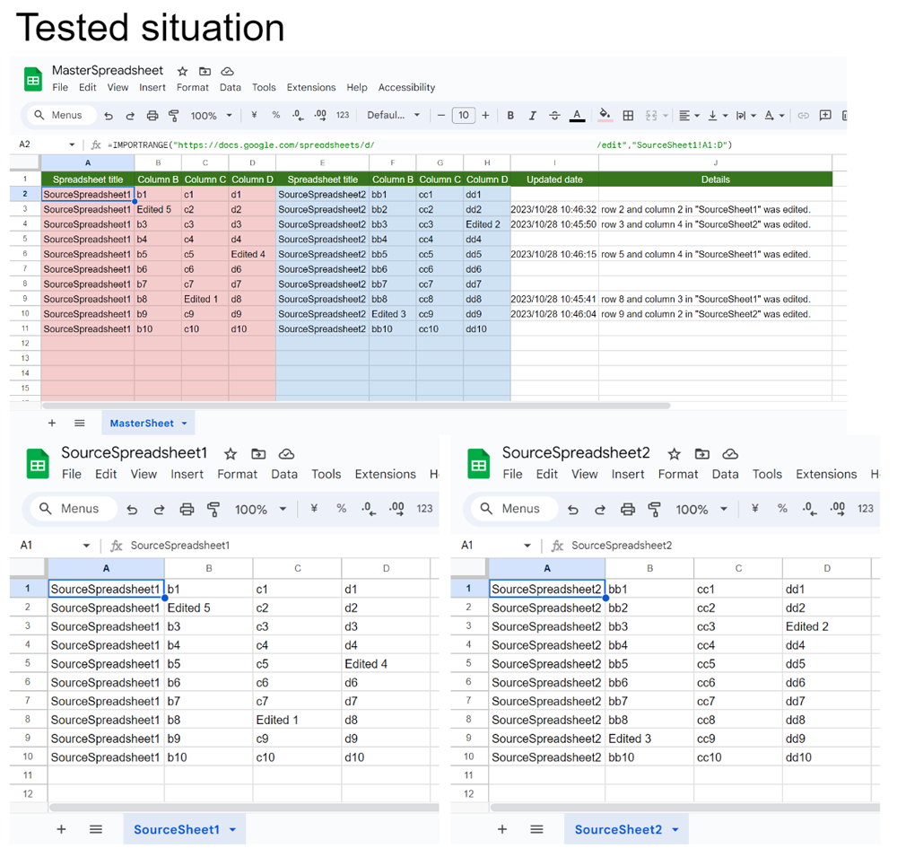
Please run main function with the script editor. By this, the installable OnEdit trigger is installed. After this, in order to test this script, please edit “SourceSheet1!A1:D” in “SourceSpreadsheet1” and “SourceSheet2!A1:D” in “SourceSpreadsheet2”. By this, you can see that the values are put into columns “I” and “J” of “MasterSheet” in “MasterSpreadsheet” with the same row of the edited row. The result situation is shown in the above image.