
Abstract
Consolidate scattered cell references (A1Notation) in Google Sheets for efficiency. This script helps select cells by background color or update values/formats, overcoming limitations of large range lists.
Introduction
When working with Google Spreadsheets, there might be a scenario where you need to process scattered A1Notations (cell addresses in the format “A1”). This could involve selecting cells with specific background colors, updating cell values, or modifying cell formats.
One approach to handle scattered A1Notations is to create a range list containing the individual cell coordinates and activate it. However, this method becomes inefficient when dealing with a large number of cells due to the high processing cost associated with activating each cell individually.
To address this limitation, consolidating scattered A1Notations into continuous ranges offers a significant performance improvement. While a previous report discussed expanding consolidated A1Notations back into individual cells Ref: https://tanaikech.github.io/2020/04/04/updated-expanding-a1notations-using-google-apps-script/, consolidating them for processing efficiency had not been covered.
During the development of a script to achieve consolidation, it became apparent that existing solutions were not straightforward. To ensure clarity and facilitate debugging in the initial stages, the script was created by splitting each step into smaller, testable functions. While this approach might appear less elegant, it prioritizes understandability during the development process.
The provided script offers a solution for consolidating scattered A1Notations, as illustrated in the demonstration image. By consolidating the notations, the script can efficiently select cells with a specific background color, reducing the overall processing cost.
Furthermore, the script’s functionality can be extended to other use cases. For instance, it can be used to update the values or formats of scattered cells across the spreadsheet.
Principle
In this script, the process of consolidating A1Notations into rectangles is achieved by calculating the maximum rectangle size for all given A1Notations. This essentially combines scattered A1Notations into a single, most efficient rectangle.
The sample situation is as follows.
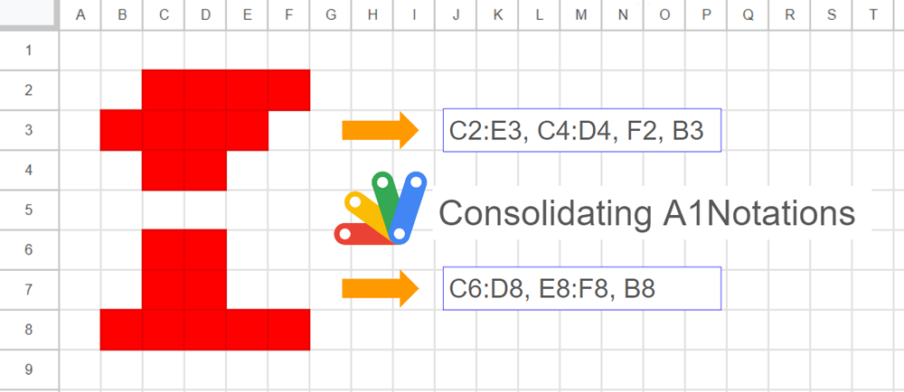
The cells with a red background color are used in this example. When the A1Notations are retrieved from those cells, it is as follows.
[
  "C2",
  "D2",
  "E2",
  "F2",
  "B3",
  "C3",
  "D3",
  "E3",
  "C4",
  "D4",
  "C6",
  "D6",
  "C7",
  "D7",
  "B8",
  "C8",
  "D8",
  "E8",
  "F8"
]
When these A1Notations are consolidated, it becomes as follows.
["C2:E3", "C6:D8", "C4:D4", "E8:F8", "F2", "B3", "B8"]
Here, the maximum size of the rectangle is calculated starting from the top-left cell (C2 in this example). This approach determines the result values in the above output order.
It’s important to note that if the situation is changed, the maximum size of the rectangle might not always be obtainable using this method. While it’s possible to modify the starting cell for calculation to ensure the maximum rectangle size is always found, this can significantly increase the processing cost. Therefore, this script adopts the top-left cell as the starting point for calculation to strike a balance between efficiency and accuracy.
The image provides a visual representation of the consolidation process applied to a sample set of A1Notations.
The script can be seen at my repository.
Usage
1. Create a Google Spreadsheet
Please create a new Google Spreadsheet. And, please set the background color as the above image. In this sample, the background colors are set in “B2:F8”.
And, please open the script editor of this Spreadsheet.
2. Install library
In this case, the script is a bit complicated. So, I added this script to my existing library UtlApp. By this, this library can expand and consolidate the A1Notations.
You can see how to install this library at here.
3. Sample script 1
In this sample, the situation of the above image is used. The script is as follows.
function sampl1() {
  const defColor = "#ffffff";
  const sheet = SpreadsheetApp.getActiveSheet();
  const backgrounds = sheet
    .getRange(1, 1, sheet.getMaxRows(), sheet.getMaxColumns())
    .getBackgrounds();
  const array = backgrounds.reduce((ar, r, i) => {
    r.forEach((c, j) => {
      if (c != defColor) {
        ar.push(`${UtlApp.columnIndexToLetter(j)}${i + 1}`);
      }
    });
    return ar;
  }, []);
  const res = UtlApp.consolidateA1Notations(array);
  Browser.msgBox(JSON.stringify(res));
}
When this script is run, the following result is obtained.
4. Sample script 2
In this sample, the following result is obtained.
The cells of the red background color are selected by this script. And, the background color of the selected cells is manually changed.
The script is as follows.
function sampl2() {
  const defColor = "#ffffff";
  const sheet = SpreadsheetApp.getActiveSheet();
  const backgrounds = sheet
    .getRange(1, 1, sheet.getMaxRows(), sheet.getMaxColumns())
    .getBackgrounds();
  const array = backgrounds.reduce((ar, r, i) => {
    r.forEach((c, j) => {
      if (c != defColor) {
        ar.push(`${UtlApp.columnIndexToLetter(j)}${i + 1}`);
      }
    });
    return ar;
  }, []);
  const res = UtlApp.consolidateA1Notations(array);
  sheet.getRangeList(res).activate();
}
IMPORTANT
- I’m worried that this method might not be able to be used on a Google Spreadsheet with a large size because of the process cost.
Note
- The top abstract image was created by Gemini from the section of “Introduction”.